This wikiHow teaches you how to find the average growth rate of an investment in Microsoft Excel. Average growth rate is a financial term used to describe a method of projecting the rate of return on a given investment over a period of time. By factoring the value of a particular investment in relationship to the periods per year, you can calculate an annualized yield rate, which can be useful in the development of an investment strategy.
StepsPart 1Part 1 of 3:Formatting Your Data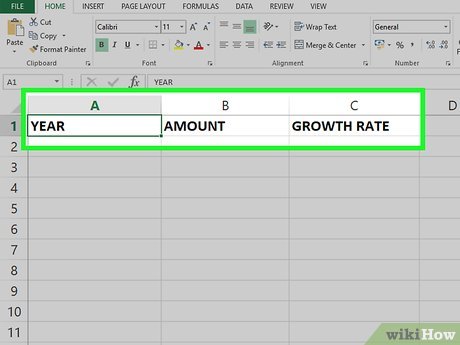
1Label your columns. The first thing we’ll need to is create column labels for our data.Type “Year” into A1 (the first cell in column A).Type “Amount” into B1.Type “Growth Rate” into C1.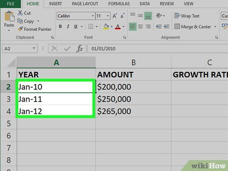
2Add the years for your investment to the Year column. Column A should contain a list of every year you’ve had the investment. In the first available cell of Column A (A2, just below the column label), type “Initial Value” or something similar. Then, in each subsequent cell, list each year.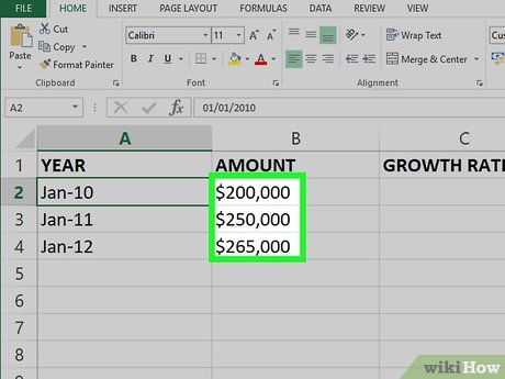
3Add the value of your investment per year to the Value column. The first available cell of Column B (B2, just below the label) should contain the amount of the initial investment. Then, in B3, insert the investment’s value after one full year, and repeat this for all other years.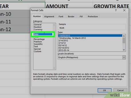
4Set the number formatting for the average growth rate calculator. To ensure your numbers display properly, you’ll need to add numerical formatting to your cells:Click column A (the letter above the column) to select it, and then click the Format button on the Home tab. It’ll be near the top-right corner of Excel. Then, click Format Cells on the menu, select Date in the left panel, and then choose a date format in the right panel. Click OK to save your changes.For column B, you’ll want to format the amounts as currency. Click the “B” above column B to select it, click the Format button on the Home tab, and then click Format Cells on the menu. Click Currency in the left panel, select a currency symbol and format on the right, and then click OK.Column C should be formatted as percentages. Click the “C” above column C, and again, click Format, and then Format Cells. Select Percentage in the left panel, choose the number of decimal places in the right panel, and then click OK.Part 2Part 2 of 3:Calculating the Yearly Growth Rate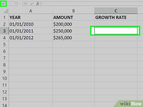
1Double-click cell C3. The reason you’re starting with this cell is because A3 represents the first completed year of your investment, and there’s nothing to calculate for the initial investment amount.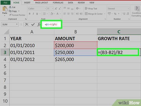
2Enter the formula for calculating the annualized yield rate. You can type this into the cell itself, or into the formula bar (fx) at the top of the worksheet: =(B3-B2)/B2
3Press ↵ Enter or ⏎ Return. This displays the growth rate for the first year of your investment in cell C3.X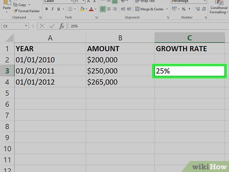
4Apply the formula to the remaining cells in column C. To do this, click the cell containing the growth rate for the first year (C3) once, and then drag the cell’s bottom-right corner downward to the bottom of your data. You can also double-click that cell’s bottom-right corner to accomplish the same task. This displays the growth rate for each year. Part 3Part 3 of 3:Calculate the Average Growth Rate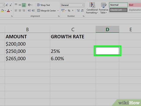
1Double-click a blank cell in a different column. This cell is where the average growth rate of your existing data will appear.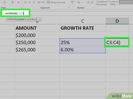
2Create a formula using the AVERAGE function. The AVERAGE function tells you the mean average of a set of numbers. If we calculate the mean average of the growth rates we calculated in column C, we’ll find the average growth rate of your investment. The column should look like this:=AVERAGE(C3:C20) (replace C20 with the address of the actual last cell containing a growth percentage in column C).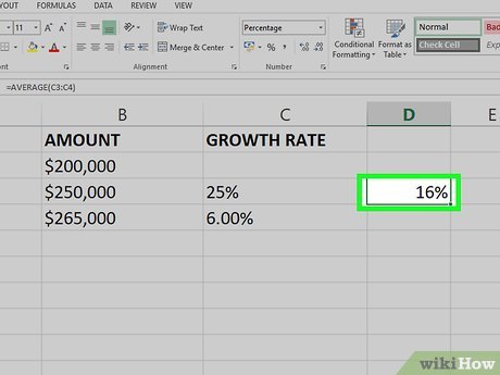
3Press ↵ Enter or ⏎ Return. The average growth rate of your investment now appears in the cell.